Nodes and the State Node model

Kathryn elaborates every Hybrid Design Block (HDB) into a graph of nodes. The three central node types are Assignment, State, and Synchronize; this page covers the complete mechanism of every node type, including the State Node’s formal execution model.

The nine node types

Each node type below carries a distinct role in the elaborated graph. Three of them — Assignment, State, and Synchronize — do the bulk of the work; the remaining six are structural or value-carrying helpers.

1. Assignment Node

A designer-issued assignment (<<= or =) to a fundamental resource or a hardware aggregator. It carries metadata such as the target UpdatePool and the associated UpdateEvent (see Driven Logic Structure). An Assignment Node does not write its target directly: it belongs to a State Node, and when that state’s operation status asserts, the node’s update event is pushed into the target’s pool, where decentralized priority resolution decides the committed value. This is the graph-level counterpart of every Cycle-Considered Operation a design writes.

2. State Node

The backbone of most HDBs and the atomic element of the HDF state machine. Each HDB instantiates its own State Nodes, and a State Node represents a single state — it orchestrates the internal nodes it owns and defines their execution conditions and connections. When a state is active it fires its Assignment Nodes and evaluates its outgoing dependencies to decide the next state. Its precise behavior is given by the formal execution model below (the os/exit signals over a dependency set, with hold, interrupt-start, and interrupt-reset inputs).

3. Synchronize Node

Used by par HDBs when the cycle usage of the parallel sub-blocks cannot be determined statically. It adds auxiliary hardware to track when each sub-block has completed and synchronizes them without spending extra cycles, so a par block advances as soon as its slowest branch finishes rather than waiting a fixed, pessimistic number of cycles.

4. Pseudo Node

A placeholder that supports cyclic node connections. When a connection must be recorded but its target node has not yet been instantiated — for example a backward edge that closes a loop — a Pseudo Node stands in for the target and is resolved to the real node once it exists. It carries no hardware of its own.

5. Dummy Node

Represents a constant value inside the node graph, so that literal constants can participate in conditions and assignment sources like any other operand.

6. Operable Node

Represents a readable hardware resource — anything derived from Operable, such as a register, wire, expression, or slot field. It is how a resource’s current value is fed into a condition or an assignment’s right-hand side; the operator expressions a design builds are trees of Operable Nodes.

7. Start Node

Auto-generated to initiate execution of the entry HDB. It provides the initial trigger that moves the top-level state machine into its first state when the design starts.

8. Wait-Condition Node

Stalls execution until a Boolean condition is satisfied. It is what the scWait(cond) construct elaborates into: the owning state holds — re-triggering itself through its hold input — until the condition becomes true, then proceeds.

9. Wait-Cycle Node

Stalls for a fixed number of cycles using a counter and its control logic. It is what syWait(N) elaborates into: the state holds for exactly N cycles before continuing.

flowchart TD
    N["HDF node types"] --> EX["execution backbone"]
    N --> VAL["value carriers"]
    N --> AUX["auxiliary"]
    EX --> SN["State Node"]
    EX --> AN["Assignment Node"]
    EX --> SY["Synchronize Node<br/>(par completion tracking)"]
    EX --> WC["Wait-Condition Node<br/>(scWait)"]
    EX --> WY["Wait-Cycle Node<br/>(syWait)"]
    VAL --> DN["Dummy Node<br/>(constants)"]
    VAL --> ON["Operable Node<br/>(readable resources)"]
    AUX --> ST["Start Node<br/>(entry HDB kick-off)"]
    AUX --> PN["Pseudo Node<br/>(cyclic connections)"]

The State Node

The State Node is the atomic element of the HDF state machine; each HDB instantiates its own State Nodes to orchestrate internal nodes and define their execution conditions and connections.

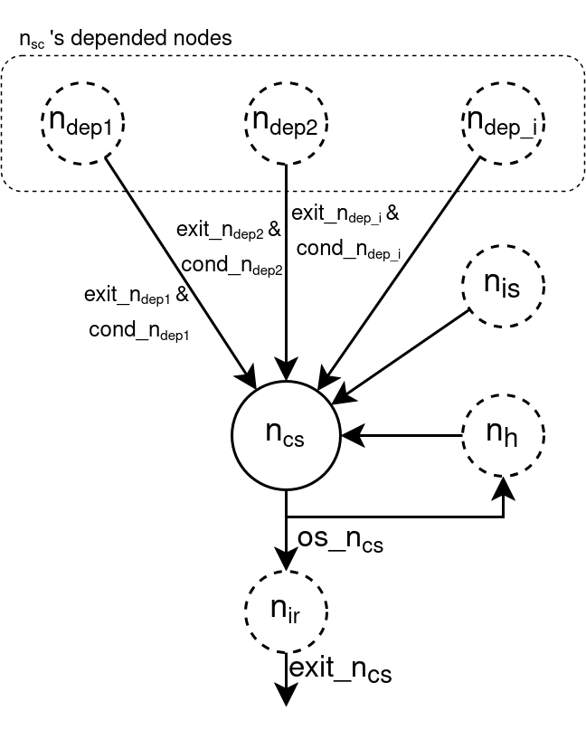
Formal execution model

The State Node’s behavior is defined over the node graph as follows:

• Node set: G = {n₁, n₂, …, n_k}

• Current state node (tuple): n_sc = (D_cs, n_h, n_is, n_ir) — dependency set D_cs; hold n_h; interrupt-start n_is; interrupt-reset n_ir.

• Exit(n_i, t) ∈ {true, false} — node n_i finishes at cycle t.

• B(c, t) ∈ {true, false} — Boolean condition c at cycle t.

• Dependency set: D_cs = {(c, n_i) | n_i ∈ G}.

• Dependency activation: Din_cs(c, n, t) = B(c, t) ∧ Exit(n, t), for (c, n) ∈ D_cs.

• Operation status:

  os_ncs(t) =
      true,   if ∃ (c, n) ∈ D_cs [ Din(c, n, t−1) ] ∨ Exit(n_is, t−1) ∨ Exit(n_h, t−1)
      false,  otherwise

• Exit status: exit_ncs(t) = os_ncs(t) ∧ Exit(n_ir, t).

Meaning: os (operation status) asserts when a preceding node, an interrupt-start node, or a hold node fired in the previous cycle, and triggers the state’s Assignment Nodes; exit gates os with the interrupt-reset signal and drives state transitions.

Note

The hold input (n_h) lets a state re-trigger itself — the mechanism behind stalling constructs — while the interrupt-start / interrupt-reset pair (n_is, n_ir) lets enclosing blocks such as pipelines start or squash a state from outside its normal predecessor chain.